12  Numpy 基础 III:标量与向量运算

12.1 标量(Scalar)

12.1.1 什么是标量?

标量是最简单的数学概念,它只有大小,没有方向。在日常生活中,我们经常遇到标量:

  • 温度:例如 25°C

  • 质量:例如 50kg

  • 时间:例如 2小时

Note

在NumPy中,单个数字就是一个标量。标量可以是整数、浮点数、布尔值等类型。

12.1.2 NumPy中的标量操作

import numpy as np

# 创建标量
x = np.float64(3.14)
y = np.int32(5)

print(f"x的类型: {type(x)}, 值: {x}")
print(f"y的类型: {type(y)}, 值: {y}")

# 标量运算
print(f"x + y = {x + y}")
print(f"x * y = {x * y}")
x的类型: <class 'numpy.float64'>, 值: 3.14
y的类型: <class 'numpy.int32'>, 值: 5
x + y = 8.14
x * y = 15.700000000000001

12.2 向量(Vector)

12.2.1 什么是向量?

向量是既有大小又有方向的量。在数学中,向量通常表示为有序的数字列表。

Tip

想象一个飞机的运动:它不仅要知道速度是多少(大小),还要知道往哪个方向飞(方向)。这就是一个向量的实际应用。

12.2.2 NumPy中的向量表示

# 创建向量
v1 = np.array([1, 2, 3])  # 3维向量
v2 = np.array([4, 5, 6])  # 另一个3维向量

print("向量v1:", v1)
print("向量v2:", v2)
向量v1: [1 2 3]
向量v2: [4 5 6]

12.3 向量运算

12.3.1 向量加减法

12.3.1.1 向量加法的概念

向量加法在物理和数学中非常常见。例如,当我们描述一个物体的运动时,可能需要把多个位移向量相加。

Note

向量加法满足以下性质: 1. 交换律:\[\mathbf{a} + \mathbf{b} = \mathbf{b} + \mathbf{a}\] 2. 结合律:\[(\mathbf{a} + \mathbf{b}) + \mathbf{c} = \mathbf{a} + (\mathbf{b} + \mathbf{c})\]

12.3.1.2 NumPy中的向量加法

# 向量加法
sum_v = v1 + v2
print(f"v1: {v1}")
print(f"v2: {v2}")
print(f"v1 + v2 = {sum_v}")
v1: [1 2 3]
v2: [4 5 6]
v1 + v2 = [5 7 9]
import matplotlib.pyplot as plt

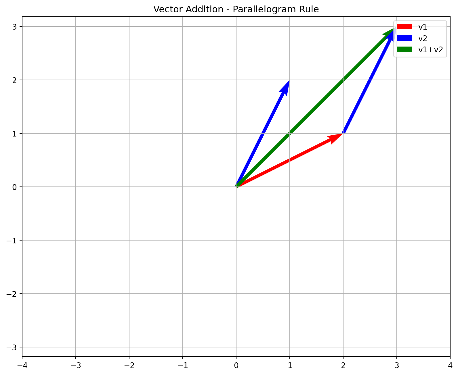
def plot_vector_addition(v1, v2):
    plt.figure(figsize=(10, 8))  # Increased figure size
    # Draw first vector
    plt.quiver(0, 0, v1[0], v1[1], angles='xy', scale_units='xy', scale=1, color='r', label='v1')
    # Draw second vector (from origin)
    plt.quiver(0, 0, v2[0], v2[1], angles='xy', scale_units='xy', scale=1, color='b', label='v2')
    # Draw sum vector
    plt.quiver(0, 0, v1[0]+v2[0], v1[1]+v2[1], angles='xy', scale_units='xy', scale=1, color='g', label='v1+v2')
    # Draw second vector (from end of first vector)
    plt.quiver(v1[0], v1[1], v2[0], v2[1], angles='xy', scale_units='xy', scale=1, color='b', linestyle='--')
    
    plt.grid(True)
    plt.axis('equal')
    # Set axis limits with padding
    max_val = max(abs(v1).max(), abs(v2).max(), abs(v1+v2).max())
    plt.xlim(-max_val-1, max_val+1)
    plt.ylim(-max_val-1, max_val+1)
    
    plt.legend()
    plt.title('Vector Addition - Parallelogram Rule')
    plt.show()

# Demonstrate 2D vector addition
v1_2d = np.array([2, 1])
v2_2d = np.array([1, 2])
plot_vector_addition(v1_2d, v2_2d)

Vector Addition - Parallelogram Rule

12.3.1.3 向量减法

向量减法可以看作是加上一个反向量:\[\mathbf{a} - \mathbf{b} = \mathbf{a} + (-\mathbf{b})\]

# 向量减法
diff_v = v1 - v2
print(f"v1 - v2 = {diff_v}")
print(f"v1 + (-v2) = {v1 + (-v2)}")
v1 - v2 = [-3 -3 -3]
v1 + (-v2) = [-3 -3 -3]

12.3.2 数乘(标量乘法)

12.3.2.1 数乘的概念

数乘是将向量的每个分量都乘以同一个标量。这个操作可以改变向量的长度,但通常不改变其方向(除非乘以负数)。

Tip

数乘的几何意义:

  • 当标量 > 1 时,向量变长

  • 当 0 < 标量 < 1 时,向量变短

  • 当标量 < 0 时,向量方向反转

# 数乘示例
scalar = 2
scaled_v = scalar * v1

print(f"原向量: {v1}")
print(f"{scalar} * v1 = {scaled_v}")
原向量: [1 2 3]
2 * v1 = [2 4 6]
def plot_scalar_multiplication(v, scalar):
    plt.figure(figsize=(10, 8))  # Increased figure size
    plt.quiver(0, 0, v[0], v[1], angles='xy', scale_units='xy', scale=1, color='r', label='Original Vector')
    plt.quiver(0, 0, scalar*v[0], scalar*v[1], angles='xy', scale_units='xy', scale=1, color='b', 
               label=f'{scalar}x Vector')
    plt.grid(True)
    plt.axis('equal')
    
    # Set axis limits with padding
    max_val = max(abs(v).max(), abs(scalar*v).max())
    plt.xlim(-max_val-1, max_val+1)
    plt.ylim(-max_val-1, max_val+1)
    
    plt.legend()
    plt.title(f'Vector Scaled by {scalar}')
    plt.show()

# Demonstrate different scalar effects
v = np.array([2, 1])
for scalar in [0.5, 2, -1]:
    plot_scalar_multiplication(v, scalar)

Effects of Scalar Multiplication

12.3.3 点积(内积)

12.3.3.1 点积的概念

点积是两个向量的一种乘法运算,结果是一个标量。其几何意义是:一个向量在另一个向量方向上的投影长度乘以另一个向量的长度。

数学表达式:\[\mathbf{a} \cdot \mathbf{b} = ||\mathbf{a}|| ||\mathbf{b}|| \cos \theta\]

Note

点积的性质: 1. 交换律:\[\mathbf{a} \cdot \mathbf{b} = \mathbf{b} \cdot \mathbf{a}\] 2. 分配律:\[\mathbf{a} \cdot (\mathbf{b} + \mathbf{c}) = \mathbf{a} \cdot \mathbf{b} + \mathbf{a} \cdot \mathbf{c}\] 3. 结合律(对标量):\[(k\mathbf{a}) \cdot \mathbf{b} = k(\mathbf{a} \cdot \mathbf{b})\]

# 计算点积
v1 = np.array([1, 2, 3])
v2 = np.array([4, 5, 6])

# 使用np.dot()计算点积
dot_product = np.dot(v1, v2)
print(f"v1 · v2 = {dot_product}")

# 计算向量夹角
cos_theta = dot_product / (np.linalg.norm(v1) * np.linalg.norm(v2))
angle = np.arccos(cos_theta)
print(f"向量夹角(弧度):{angle}")
print(f"向量夹角(角度):{np.degrees(angle)}")
v1 · v2 = 32
向量夹角(弧度):0.2257261285527342
向量夹角(角度):12.933154491899135
def plot_dot_product(v1, v2):
    plt.figure(figsize=(10, 8))  # Increased figure size
    # Draw vectors
    plt.quiver(0, 0, v1[0], v1[1], angles='xy', scale_units='xy', scale=1, color='r', label='v1')
    plt.quiver(0, 0, v2[0], v2[1], angles='xy', scale_units='xy', scale=1, color='b', label='v2')
    
    # Calculate projection
    proj_length = np.dot(v1, v2) / np.linalg.norm(v2)
    v2_unit = v2 / np.linalg.norm(v2)
    proj = proj_length * v2_unit
    
    # Draw projection
    plt.quiver(0, 0, proj[0], proj[1], angles='xy', scale_units='xy', scale=1, color='g', label='Projection')
    plt.plot([v1[0], proj[0]], [v1[1], proj[1]], '--k')
    
    plt.grid(True)
    plt.axis('equal')
    
    # Set axis limits with padding
    max_val = max(abs(v1).max(), abs(v2).max(), abs(proj).max())
    plt.xlim(-max_val-1, max_val+1)
    plt.ylim(-max_val-1, max_val+1)
    
    plt.legend()
    plt.title('Geometric Interpretation of Dot Product')
    plt.show()

# Demonstrate dot product geometry
v1_2d = np.array([2, 1])
v2_2d = np.array([1, 2])
plot_dot_product(v1_2d, v2_2d)

Geometric Interpretation of Dot Product

12.3.4 向量的性质

12.3.4.1 向量的模(长度)

# 计算向量的模
magnitude_v1 = np.linalg.norm(v1)
print(f"向量v1的模: {magnitude_v1}")
向量v1的模: 3.7416573867739413

12.3.4.2 向量的单位化

# 向量单位化
unit_v1 = v1 / np.linalg.norm(v1)
print(f"单位向量: {unit_v1}")
print(f"单位向量的模: {np.linalg.norm(unit_v1)}")  # 应该接近1
单位向量: [0.26726124 0.53452248 0.80178373]
单位向量的模: 1.0

12.3.5 实际应用示例

12.3.5.1 物理学中的位移计算

# 一个物体的运动
initial_position = np.array([0, 0, 0])  # 初始位置
displacement = np.array([3, 4, 0])      # 位移向量

final_position = initial_position + displacement
distance = np.linalg.norm(displacement)

print(f"位移向量: {displacement}")
print(f"移动距离: {distance}")
位移向量: [3 4 0]
移动距离: 5.0

12.3.5.2 计算两点之间的距离

# 平面上两点之间的距离
point1 = np.array([1, 2])
point2 = np.array([4, 6])

distance = np.linalg.norm(point2 - point1)
print(f"两点之间的距离: {distance}")
两点之间的距离: 5.0

12.3.6 练习题

  1. 给定向量 a = [1, 2] 和 b = [3, 4],计算:

    • a + b
    • a - b
    • 2a
    • a · b
  2. 计算向量 [1, 1] 和 [1, 0] 之间的夹角。

  3. 验证点积的交换律:计算 a · b 和 b · a。

a = np.array([1, 2])
b = np.array([3, 4])

print(f"a + b = {a + b}")
print(f"a - b = {a - b}")
print(f"2a = {2 * a}")
print(f"a · b = {np.dot(a, b)}")
a + b = [4 6]
a - b = [-2 -2]
2a = [2 4]
a · b = 11

12.4 小结

  • 标量是只有大小没有方向的量
  • 向量是既有大小又有方向的量
  • NumPy提供了丰富的函数来处理向量运算
  • 向量运算在物理学、工程学等领域有广泛应用
  • 向量加减法遵循平行四边形法则
  • 数乘可以改变向量的大小和方向
  • 点积是两个向量的乘法运算,结果是标量